
Visual Migration Flows: Design Your IFS Migration on a Canvas
October 30, 2026 · 10 min read
Why migration plans used to live in several places
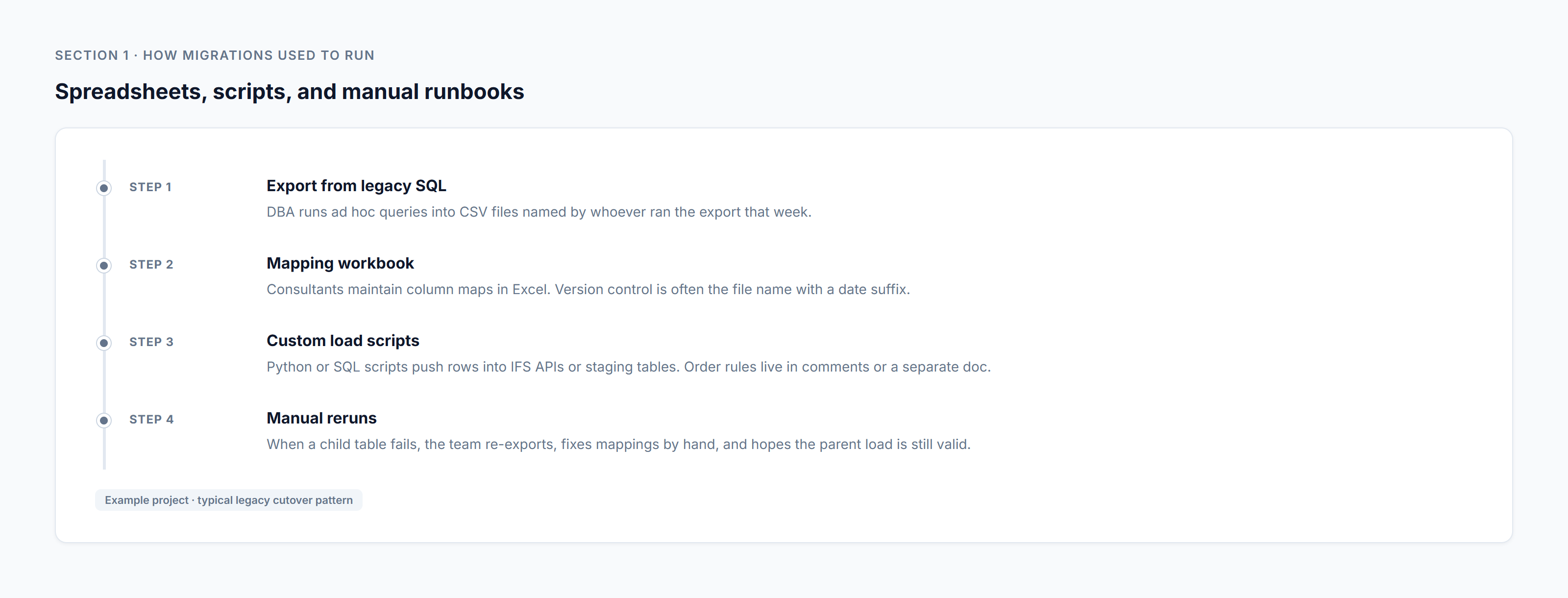
An IFS migration often starts with a sensible collection of working files:
- SQL extracts or CSV exports from the legacy system
- an Excel workbook that maps legacy columns to IFS attributes
- scripts that clean values and call IFS APIs
- a runbook that tells the cutover team which script runs first
- ticket comments that explain exceptions found during testing
Each item solves a real problem. The difficulty is that the complete migration only exists when somebody combines all five in the correct order.
Consider a customer migration with three source tables:
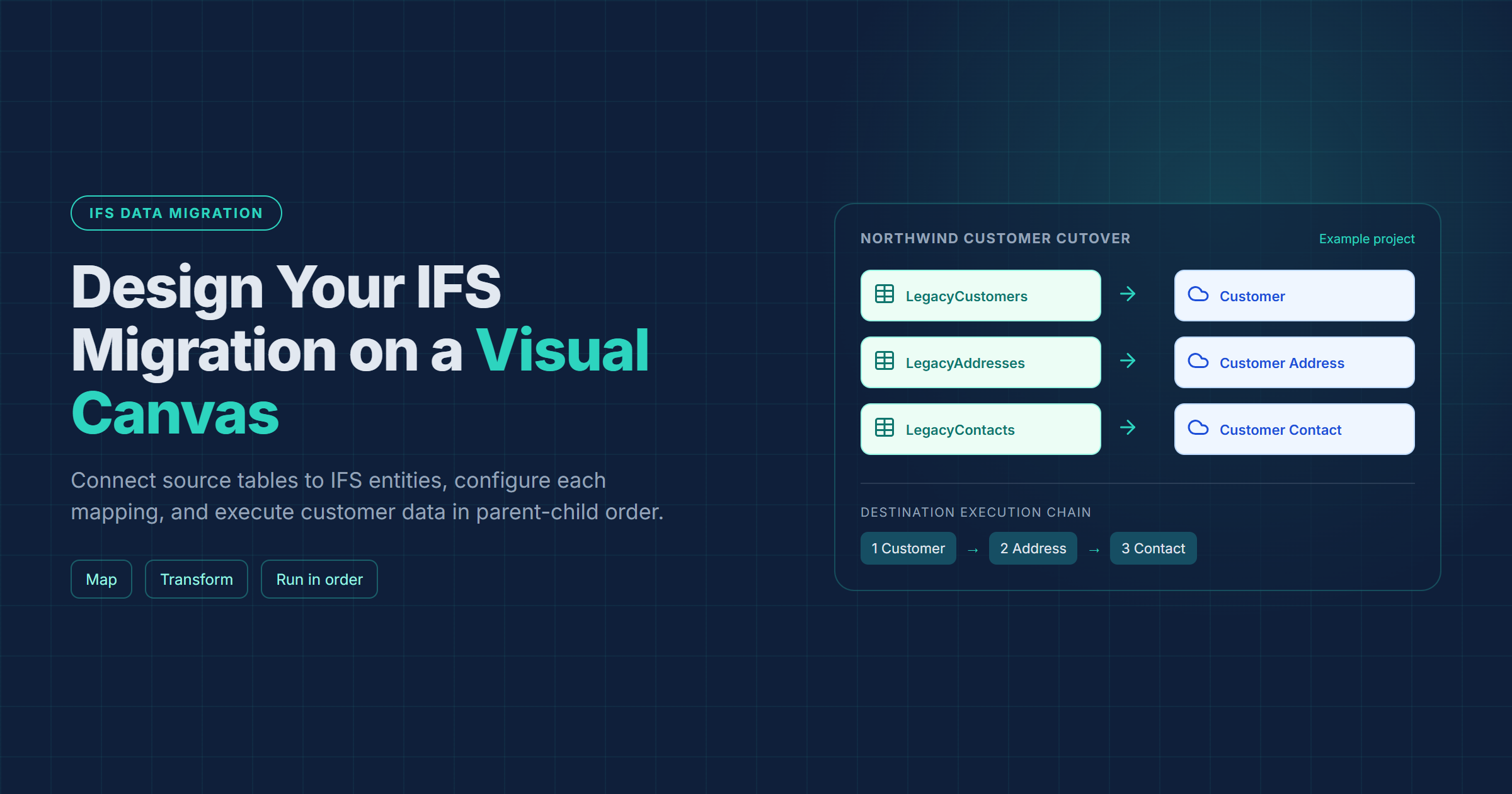
| Source table | Destination entity | Dependency |
|---|---|---|
LegacyCustomers | Customer | First |
LegacyAddresses | Customer Address | After Customer |
LegacyContacts | Customer Contact | After Customer Address |
The customer row creates the parent identity used by its addresses. Contact data may depend on both the customer and address context. If a runbook step is missed, IFS can reject child rows or leave the team with a partial load that needs investigation.
What becomes difficult as the project grows
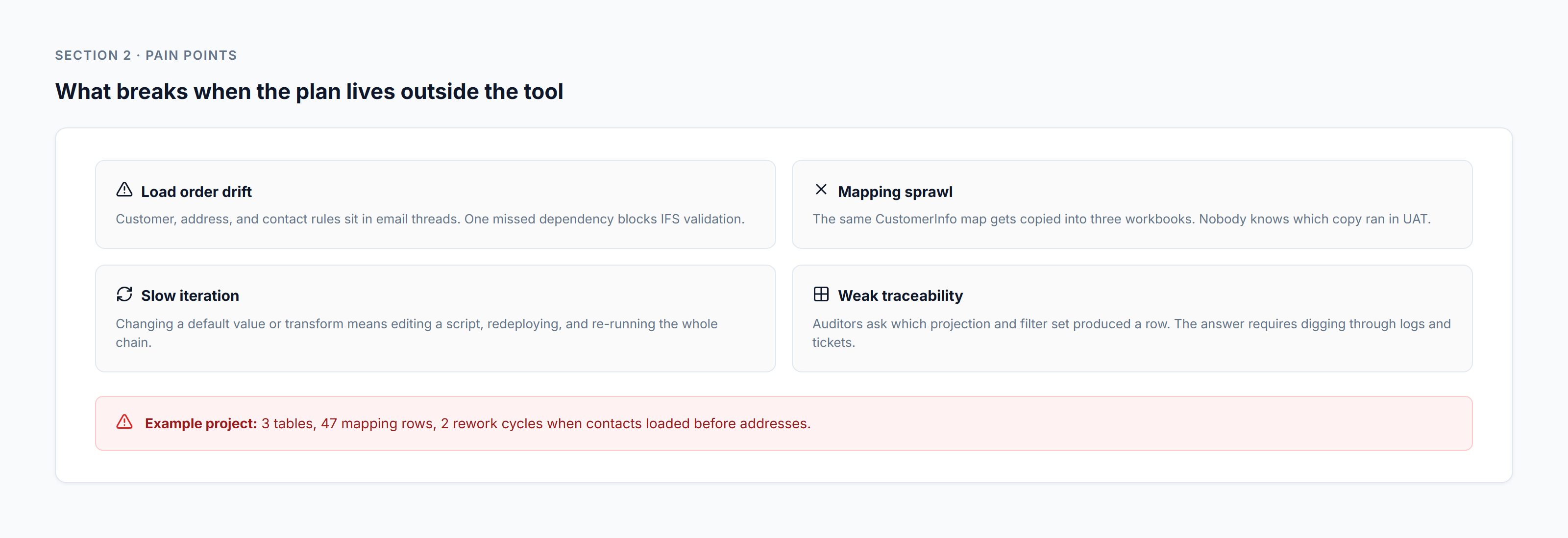
The first trial load can succeed even with a manual process. Repeated UAT cycles expose the weaknesses.
Execution order is separate from the mapping
The mapping workbook explains how CustNo becomes CustomerId, but it rarely controls when Customer Address may start. That rule sits in another document. A correct map can still be executed in the wrong sequence.
Changes are hard to trace
A consultant may change a country conversion in Excel while a developer changes the equivalent rule in SQL. The next run depends on which version is used. Reconstructing the exact configuration later takes time.
Pilot scope drifts between tables
A team may want to migrate only Northwind Engineering Ltd and customer C10042 during a pilot. If each extract has its own WHERE clause, one table can include a wider set of customers than the others.
Reruns require coordination
When an address upload fails, the team must decide whether the parent load is still valid, whether the source extract changed, and which scripts can safely run again. The answer is often held by one person rather than recorded in the migration design.
IFS API details stay hidden in scripts
The destination projection and entity set matter. If those choices are buried in code, a functional consultant cannot inspect the complete path from a legacy column to the IFS endpoint.
The canvas becomes the migration plan
C8 Data Migration Tool places the tables, mappings, and execution dependencies on a Migration Flow canvas.
Open Migration Flows, create a flow, and use the table panel on the left. The available pools in the designer are:
- IFS Source
- Custom tables
- Custom views
- IFS Destination
- Atom Source, when Atom sources are enabled
You can drag an available table onto the canvas. The table row also provides + Add, which is useful when working with a long list.
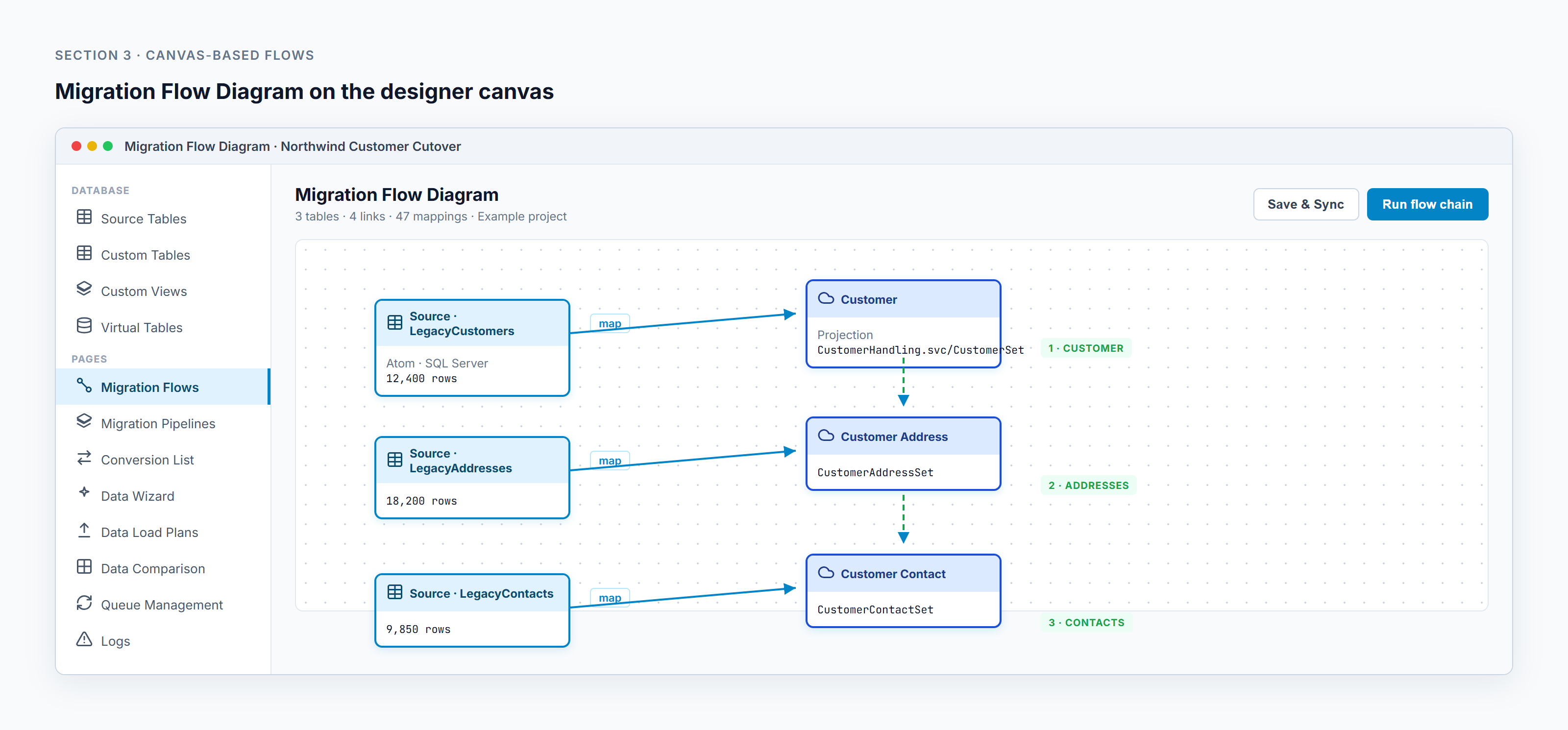
For the example project, add LegacyCustomers, LegacyAddresses, and LegacyContacts as sources. Then add the Customer, Customer Address, and Customer Contact destination entities from IFS Destination.
The result is a diagram with two kinds of connections:
- Mapping links connect a source node to the destination that receives its data.
- Flow-chain links connect one destination to the next and define execution order.
That distinction is important. LegacyAddresses → Customer Address says where address fields go. Customer → Customer Address says the address upload waits for the customer upload to finish.
A practical walkthrough: customer, addresses, then contacts
1. Add the source and destination nodes
Start with the source table pool that matches the data location. Legacy data already held in DMT can come from Custom tables or Custom views. An on-premises table exposed through a configured Atom appears under Atom Source. Live IFS entities appear in the IFS pools.
Drag the three source tables to the left side of the canvas. Add their destination entities to the right. Keeping sources and destinations in columns makes the data path easy to review, although node position does not determine execution order.
2. Run Save & Sync before mapping
The designer toolbar includes Save & Sync. It saves the flow and synchronizes the IFS source and destination tables currently on the canvas. DMT uses the synchronized metadata when it opens tables and builds mappings.
Run it after adding or changing tables. A node that has not been synchronized can remain unavailable for table-level work until synchronization completes.
3. Draw the mapping links
Connect LegacyCustomers to Customer. The Entity Mapper opens for that source-destination pair. Repeat the process for addresses and contacts.
The mapping edge stores the relationship between one source node and one destination node. Drawing a link does not finish the mapping by itself. Review the fields in the Entity Mapper and save the mapping.
4. Draw the destination chain
Connect Customer to Customer Address using the flow handles. Then connect Customer Address to Customer Contact.
The chain now reads:
Customer → Customer Address → Customer Contact
During upload, a child destination is queued until its upstream destination finishes. The execution code follows destination-chain edges and starts child sources in that sequence.
5. Upload from the destination nodes
A destination node shows its upload action after at least one linked source has saved mappings. Starting from the first destination runs the connected chain. The active handoff edge is highlighted as execution moves from one destination to the next.
Use the node log action and the shared log panel to inspect progress. Queue Management is available for migration job monitoring, including queue health and requeueing dead-letter jobs.
What you can configure in the flow
Mapping fields to IFS attributes
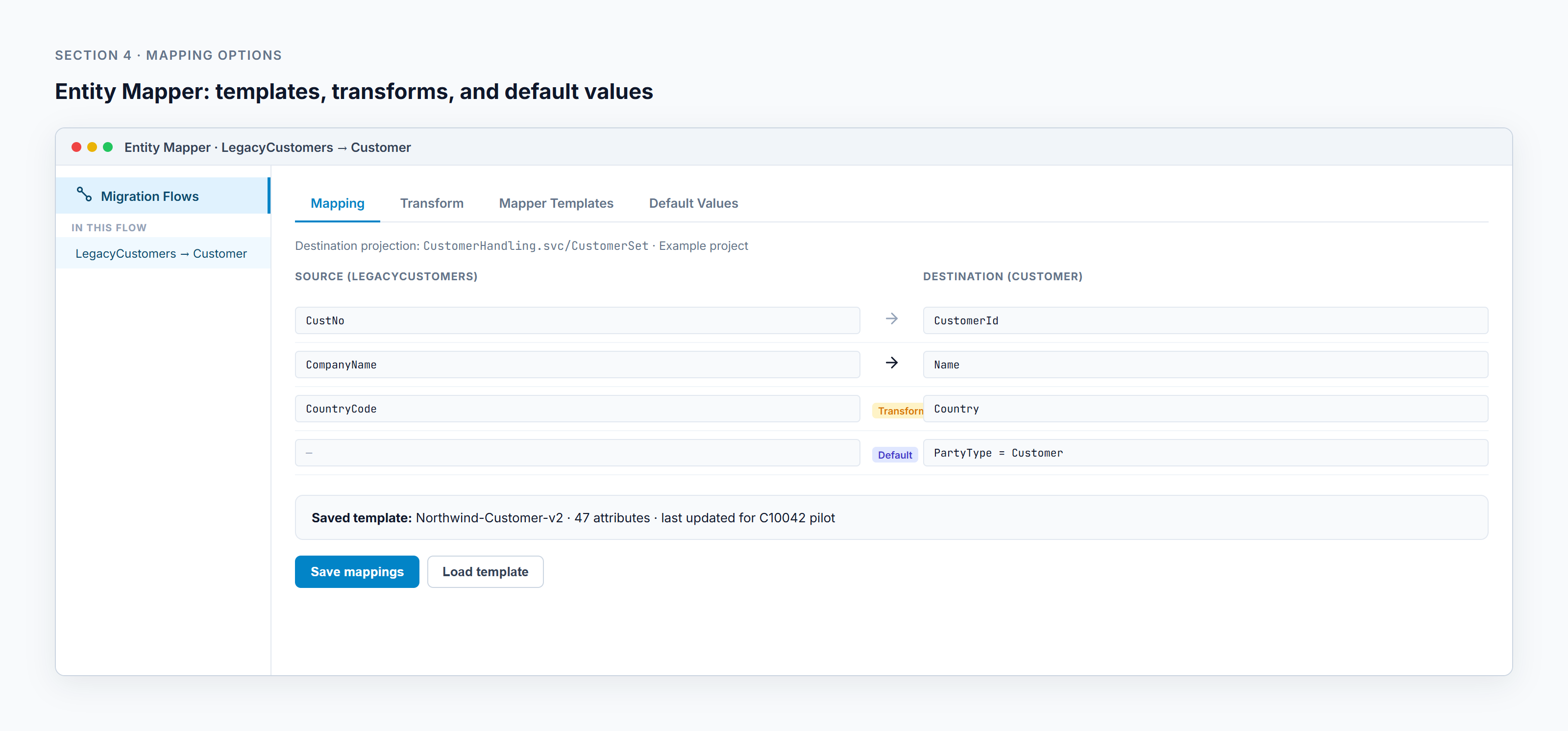
The Entity Mapper matches source fields to destination attributes. For the customer example:
| Source field | Destination attribute | Rule |
|---|---|---|
CustNo | CustomerId | Direct |
CompanyName | Name | Direct |
CountryCode | Country | Transform |
| no source field | PartyType | Default value |
Direct mappings preserve a field value. A transform prepares the value before mapping. A default fills an attribute that has no useful source field.
Selecting the destination projection
The mapper has a Destination Projection selector. DMT discovers projection options for the destination entity and records the selected projection on the flow node.
The projection controls the IFS API shape used for the destination. Review it before saving mappings, especially when an entity has several active projections or when a preferred projection changes between environments.
Reusing mapper templates
Mapper Templates save a set of source-to-destination pairs for later use. In a migration flow, template choices are scoped to the relevant flow, source table, destination entity, and destination node.
Templates help when several dry runs use the same mapping. They also help when a link is removed and later reconnected. The flow keeps mapping templates when an edge is disconnected, allowing the saved work to be restored.
Setting default destination values
Destination nodes expose Defaults in the node header. Use it for attributes that should receive a constant value, such as a party type, language code, or company value that is absent from the source.
Defaults belong to the destination mapping context and can be reviewed before upload. DMT also records who last set a default value so editing permissions can be enforced.
Shaping source data with transforms, queries, and views
Some migrations need more than one-to-one column mapping. Legacy data may use old codes, split a value across columns, or require a join to a lookup table.
The mapper presents three stages:
- Transform: shape the data visually or in SQL
- Views: materialize the result so it can transfer
- Mapping: match the resulting columns to the destination
The Transform stage supports a visual query builder. Visual and SQL are two representations of the same query. The visual builder can select columns, add joins, define filters, and preview the result. Free-form SQL is available only when the corresponding configuration is enabled.
For example, a customer transform could:
- select
CustNo,CompanyName, andCountryCode - join a country conversion table
- filter out inactive legacy customers
- output
CustomerId,Name, and a normalizedCountry
After the transformed result is materialized as a view, the Mapping stage uses the view's output columns. This keeps transformation logic attached to the source-destination path instead of hiding it in an unrelated deployment script.
Keeping the pilot scope consistent with Global Filters
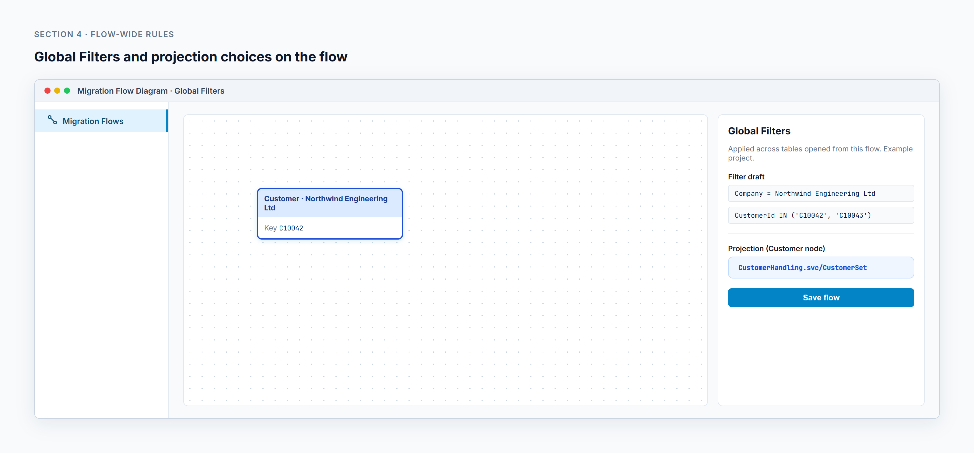
The Global Filters tab builds attribute-based rules across the migration flow. A rule contains an attribute, an operator, and one or more values. The available attributes come from tables already added to the canvas.
For an example pilot, define:
Company = Northwind Engineering Ltd
CustomerId IN (C10042, C10043)
The chain execution converts the configured global rules into API filters and uses the consolidated filters for download and upload. This gives the three-table chain a common scope.
Global filters still require careful field selection. The participating tables need attributes that allow the same business scope to be expressed. Review the filtered rows before a production run.
Saving, running, and checking the result
A reliable flow run follows a short sequence:
- Add source and destination nodes.
- Run Save & Sync after table changes.
- Create each source-to-destination mapping.
- Confirm projections, transforms, views, templates, and defaults.
- Connect destination nodes in parent-child order.
- Apply Global Filters for a pilot or limited run.
- Upload from the first destination in the chain.
- Review logs and Queue Management.
- Use Data Comparison when row-level source and destination comparison is required.
The diagram gives reviewers a single place to answer practical questions. They can see which source feeds Customer, which projection is selected, whether an edge has a transform, and which destination waits for its parent.
How this changes the migration workflow
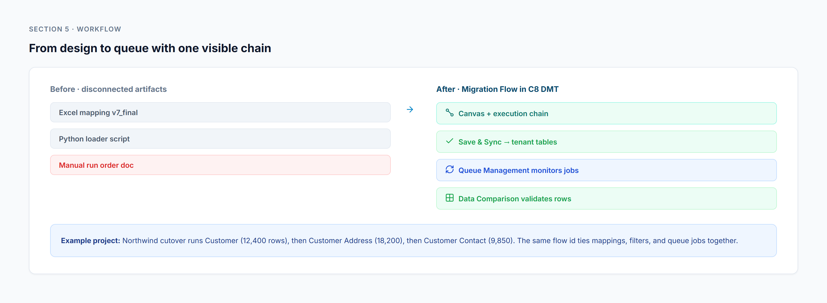
The canvas shortens the distance between design and execution.
A functional consultant can review table relationships and destination order without reading a loader script. A developer can open the Transform stage and inspect the visual query or SQL. A test lead can use the same flow during each UAT cycle and compare results without rebuilding the runbook.
It also makes change review more specific. Instead of saying "the customer migration changed," the team can identify the exact change:
- the destination projection changed
- a mapping template was updated
- a default value was added
- a transform join was revised
- the global pilot filter changed
- a destination was moved in the execution chain
Canvas locking is available to Super Admins when a flow should remain read-only for other users. Prebuilt flows can provide a starting template, while flow bundle export and import can move the full diagram and its associated transform plans.
Bottom line
A visual migration flow gives the IFS cutover team one executable description of the migration. Sources, destinations, mappings, projections, transforms, defaults, filters, and dependency order stay connected.
For the customer example, the logic is visible from left to right and top to bottom: LegacyCustomers maps to Customer, LegacyAddresses maps to Customer Address, and LegacyContacts maps to Customer Contact. The destination chain controls the order: customer first, addresses second, contacts third.
That clarity matters during repeated test cycles. The team can inspect the plan, change one part, save it, and run the same defined chain again with logs and queue activity tied to the flow.